机器学习基础

Machine Learning can be divided to :
- supervised learning
- unsupervised learning

Supervised learning

Needs data set with labels

TO: predict unknown future output

• Classfication Problem (discrete): to predict a discrete output (say yes or no), e.g Cancer benign or malignant diagnosis

• Regression Problem (Continous): to predict a specific number, e.g Stock Price Prediction

During a linear regression problem we have to solve a minimization problem, to minimize the difference between $x$ and $h(y)$.

Regression Problem

Training set + learning algorithm -> generate hypothesis function $h$

$h$ takes input $x$ (e.g. size of house) and output $y$ (e.g. estimated selling price)

Cost Function:

$$J(\theta_{0},\theta_{1})=\frac{1}{2m} \Sigma (h_{\theta}(x)-y)^2$$

Sigma from 1 to m (m equal to sample size)

Gradient Descent

repeat until convergence:

$$\theta_j := \theta_j -\alpha\frac{\partial}{\partial \theta_j}J(\theta_0 , \theta_1)$$

(for $j$ = 0 and $j$ = 1)
:= means denote assignment
$\alpha$:learning rate, basically controls how big is a step when descent
$\theta_0$ and $\theta_1$ have to be updated simultaneously

Linear Regression Algorithm

TO: Apply gradient descent algorithm to minimize squared error cost function

“Batch” gradient descent: each step of gradient descend uses all training examples

Multiple features (variables)

Hypothesis:$h_\theta (x) = \theta_T x = \theta_0 x_0 + \theta_1 x_1 ... + \theta_n x_n$
Parameters:$\theta_0,\theta_1,...,\theta_n$
Cost function:

$$J(\theta_0,\theta_1,...,\theta_n) = \frac{1}{2m}\Sigma (h_\theta(x^{(i)})-y^{(i)})^2$$

Sigma from i=1 to m

Gradient descent:
repeat fellow:

$$\theta_j := \theta_j -\alpha\frac{\partial}{\partial \theta_j}J(\theta_0 , \theta_1)$$

(simutaneously update for every $j$)

As a result new algorithm will be like fellow:

$$\theta_j := \theta_j - \alpha \frac{1}{m} \Sigma (h_\theta(x^{(i)})-y^{(i)})^2 x_j^{(i)}$$

(simultaneously update $\theta_j$ for $j=0,1，...,n$)
E.g from a data set with three features it may like follows:

$$\theta_0 := \theta_0 - \alpha \frac{1}{m} \Sigma (h_\theta(x^{(i)})-y^{(i)})^2 x_0^{(i)}$$

$$\theta_1 := \theta_1 - \alpha \frac{1}{m} \Sigma (h_\theta(x^{(i)})-y^{(i)})^2 x_1^{(i)}$$

$$\theta_2 := \theta_2 - \alpha \frac{1}{m} \Sigma (h_\theta(x^{(i)})-y^{(i)})^2 x_2^{(i)}$$

Feature Scaling & Mean normalization

Idea:make sure features are on a similiar scale.

E.g. $x_1$ = size (0-2000 feet^2) while $x_2$ = number of bedrooms (1-5)

Learning rate

• if $\alpha$ is too small: slow convergence
• if $\alpha$ is too large: $J(\theta)$ may not decrease on every iteration; may not converge

Make sure gradient descent is working correctly.Final goal is converge the cost function.

Features and Polynomial Regression

E.g. Housing prices prediction

$$h_\theta (x) = \theta_0 + \theta_1 \times frontage + \theta_2 \times depth$$

Clearly frontage is the first feature $x_1$ and depth is the second feature $x_2$

To decide which feature is the most important factor to the housing price, thereafter a polynomial regression can be taken:

$$h_\theta (x) = \theta_0 + \theta_1 \times frontage + \theta_2 \times depth^2$$

this formula can be written as:

$$h_\theta (x) = \theta_0 + \theta_1 \times x_1 + \theta_2 \times x_2^2$$

In this case, feature scaling is becoming increasingly important to get them comparable.

Classification Problem (Discrete)

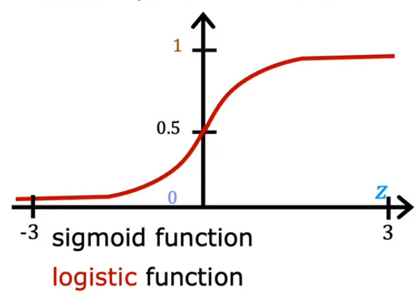
Sigmoid Function

Want outputs 0 or 1

Sigmoid Function(Logistic Function):

$$g(z)= \frac{1}{1+e^{-z}}$$

while $z$ can be written as vector($\vec{w}$ is weights and $x$ is feature):

$$z = \vec{w}x + b$$

Decision Boundary

$$f_{\vec{w},b}(x) = g(\vec{w}x+b) = \frac{1}{1+e^{-(\vec{w}x+b)}}=P(y=1|x;\vec{w},b)$$

Clearly the decision boundary is the threshold value of $f_{\vec{w},b}(x)$.

$x$ is also can be replaced by $\vec{x}$ if there are multiple features.

Clearly the descision boundary is

$$\vec{w}x+b=0$$

Cost Funciton

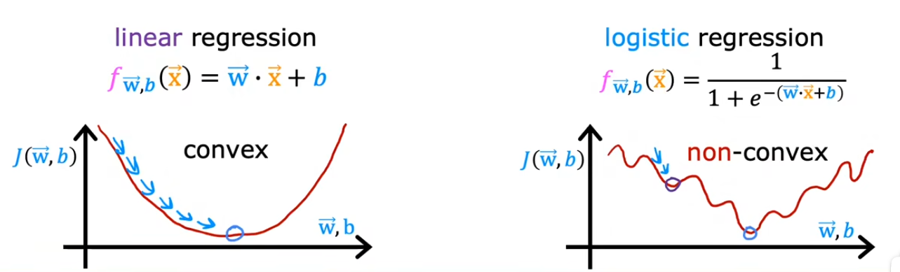
Since MSE under logistic regression is a non-convex function, using MSE as cost function index may get “stuck” at the inflection point of the function, causing error.

Target:create or select a new cost function to make it convex.

The loss function of logistic regression uses the log-likelihood loss function, also known as the cross-entropy loss function, which is used to measure the difference between the model prediction and the true label. The loss function is defined as:

$$L(\theta) = - \frac{1}{m} \sum_{i=1}^{m} \left[ y^{(i)} \log h_{\theta}(x^{(i)}) + (1 - y^{(i)}) \log (1 - h_{\theta}(x^{(i)})) \right]$$

while

• $m$:sample amounts
• $y^{(i)}$: true label (0 or 1) of sample $i$
• $h_{\theta}(x^{(i)})$: The model predicts the probability of sample $i$, i.e. $P(y=1|x^{(i)})$

The goal of this loss function is to minimize the gap between the predicted and actual labels.

Training Logistic regression

Use gradient descent to minimize the cost function $J(\vec{w},b)$.

we have

$$\frac{\partial}{\partial w_j} J(\vec{w},b) = \frac{1}{m} \sum_{i=1}^{m} \left[ f_{\vec{w},b}(\vec{x}^{(i)}-y^{(i)})\right]x_j^{(i)}$$

and

$$\frac{\partial}{\partial b} J(\vec{w},b) = \frac{1}{m} \sum_{i=1}^{m} \left[ f_{\vec{w},b}(\vec{x}^{(i)}-y^{(i)})\right]$$

what we need to do is update them simultaneously.

Unsupervised learning

Needs data set without labels

TO: Automatically discover the internal patterns or structures of data, such as dividing data into different clusters, revealing the inherent laws of data, or simplifying data representation.

Example : Extracting vocals from audio

决策树(Decision Tree)

E.g.：判断动物是否为猫

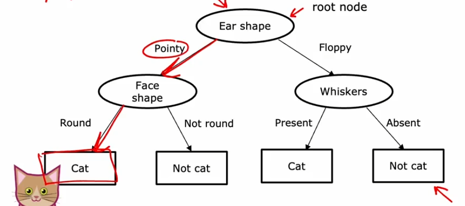
决策树训练步骤

• 确认第一个决策节点(Node)后对样本进行分类 例如：待检测动物的耳朵是圆的还是尖的
• 确认剩下的节点

需要解决的问题

• 如何确定每个节点所用来进行分类的特征(Feature)？如：是根据耳朵类型进行分类还是根据体型进行分类
• 什么时候停止继续分类（split）？
  • 某节点能够做到100%的分类时（如有猫DNA的动物一定是猫，不可能是其他）
  • 某节点之后决策树溢出
• 继续进行决策所带来的提升低于阈值
• 节点中的样本数量过少